Contents

1 Introduction

To date, the Nock combinator calculus or instruction set (depending on one’s viewpoint) has been evaluated using either a tree-walking interpreter or a bytecode interpreter. The former has been found straightforward to implement but regrettably slow in practice. Following a suggestion by ~ritpub-sipsyl to incorporate better information about what is known about the subject into the compilation process, Urbit engineers elaborated Subject Knowledge Analysis, or ska. This static analysis pass is performed on a subject-formula pair, producing a call graph and a subject mask. The latter can be used to determine if two subject-formula pairs are equivalent, allowing the reuse of analysis results. The call graph can be used to introduce direct calls in the bytecode interpreter, as well as to perform compile-time jet matching. ska unlocks ample gains in practical Nock performance, as well as enabling future optimizations and analyses.

2 Dynamism of Nock

The Nock 2 operator is one of the two opcodes that are used for Nock evaluation. From the Nock specification:

*[a 2 b c]          *[*[a b] *[a c]]

Put plainly, we evaluate two operands of Nock 2 against the given subject, then evaluate Nock with the product of the first operand as a subject, and the product of the second operand as a formula.

The compound Nock 9 operator is defined in terms of other Nock operators:

*[a 9 b c]          *[*[a c] 2 [0 1] 0 b]

Evaluation of the formula from the second operator yields a noun, from which a formula to be evaluated is pulled with Nock 0. That formula is then evaluated against that noun, which is often referred to as a “core”.

Since Nock 9 is essentially a macro for Nock 2, we can focus our attention on Nock 2. This operator is equivalent to eval in other languages: execution of dynamically generated code. Unlike most languages, Nock does not have a notion of a static call, and all function calls are implemented in terms of eval. In practice, however, we can discover formula products *[a c] for almost all Nock 2 sites, given the subject.

Examples when we cannot do that, such as receiving code to evaluate over the wire, or from the outer virtualization context via Nock 12, or as a product of a complex expression where we cannot reliably execute it at compile time, are rare. In practice, these exceptions are limited to either evaluating dynamically-supplied code or running the Hoon compiler at run time, e.g. in vase mode.¹ For all other cases, e.g. Arvo, Gall agents, the subject’s code contents do not often change and the result of static analysis is likely to be reused until a kernel upgrade or Gall agent upgrade respectively.

This static analysis procedure, dubbed “Subject Knowledge Analysis”, is as follows: given a pair of a subject and a formula, we construct the call graph for all Nock 2 sites for which we have enough information, yielding call graph information and subject mask. A new subject-formula pair where the formula is equal to the analyzed formula, and the parts of the subject included in the mask are equal to the same parts from the previously analyzed subject, is considered to be equivalent. Consider analyzing the subject-formula pair:

[[dec 1] [%9 2 %10 [6 %0 3] %0 2]]

Then a pair [[dec 2] [%9 2 %10 [6 %0 3] %0 2]] is equivalent to the first one in terms of the call graph information: the different subnouns of the subject are never used as code by the $ arm of the dec core. A pair of a minimized subject and a formula thus constructs an object equivalent to a function in other languages, with the masked out parts of the subject being the function’s arguments. Further in the text, we will refer to pairs (minimized subject)-formula as functions that we discovered during the analysis.

3 Motivation

In prior work on ska by ~ritpub-sipsyl and ~master-morzod, the analysis was considered as a first step in compiling Nock to a static single assignment intermediary representation language (ssa ir) to introduce direct calls in Nock. In their absence, Nock registerization, or any kind of optimization/analysis for that matter is limited by the lack of knowledge about the call target and the call product: in the ssa ir example, we would not know which parts of a call’s subject are actually used by the callee program.

For the current work, a simpler goal was set: the introduction of direct calls and compile-time jet matching in the Vere bytecode interpreter. Currently, the interpreter has to, first, look up a Nock bytecode program in the bytecode cache, and second, it has to dynamically perform a jet matching routine at each Nock 9 call site.² With ska, the bytecode programs could have instructions for direct calls into other bytecode programs, and a program could also check if a given Nock 2 site matches some jet information the program has already accumulated, thus adding the jet driver directly into the bytecode stream if the match was obtained.

4 Core Algorithm

To analyze a subject-formula pair, we run what is essentially a partial Nock interpreter to propagate known information to formulas deeper in the formula tree, and to accumulate call graph information. Instead of a noun, the subject is a partial noun described with the type $sock:

+$  cape  $~(| $@(? [cape cape])) 
+$  sock  $~([| ~] [=cape data=*])

That is, $cape is a mask that describes the shape of the known parts of a given noun, and $sock is a pair of a mask and data, where unknown parts are stubbed with 0 or ~.

The treatment of the partial noun by that interpreter is mostly trivial:

• Autocons conses the partial products, normalizing the mask and data if necessary.

• Nock 0 grabs a subnoun from $sock if it can, otherwise it returns unknown result [| ~].

• Nock 1 returns a fully known result.

• Actual computations (Nock 3, Nock 4, and Nock 5) return unknown result [| ~] – we do not attempt to run all code at compile time, we just want to evaluate code-generating expressions.

• Nock 6 produces an intersection of the results of branches, that is, only parts of the products that are known and equal between branches.

• Nock 7 composes formulas: the product of the first formula is passed as a partial subject to the second one.

• Nock 10 edits the product of one formula with the product of the other. If the recipient noun is not known, and the donor noun is known at least partially, cells will be created that lead to the edited part.

• Nock 8 and Nock 9 are desugared in terms of Nock 7, Nock 2, and autocons.

• Nock 11 calls have their dynamic hint formula products dropped and some hints are handled directly.

  • %spot hints are used for debugging/verbose printouts.

  • %fast hints are used to accumulate cold state.

• Nock 12 of the virtual Nock produces an unknown result.

In the case of Nock 2, the operands are evaluated, and then we check if the formula at this site is fully known. If it is not known, the call is indirect – we cannot make any assumptions about its product, so we return [| ~]. If it is known, we do two things:

1. We record information on subject usage as code for each call below us in the stack, including the root call. This step is needed to produce a minimized subject for each call, which is necessary to avoid redoing the work for the functions we already analyzed.

2. We enter a new frame of the partial interpreter, executing/analyzing new $sock–formula pair we just got, returning the result of that analysis as a product.

To track the code usage of the subjects of function calls, the partial noun is paired with a structure to describe the flow of data from the functions below us in the stack to the new callsite. That data structure will be described later in the performance section.

5 Loop handling

The most complicated part of the algorithm is the handling of loops. Unlike the regular interpreter, where only one branch is executed at a time, the partial interpreter enters both, so a lack of loop handling would quickly lead to an infinite cycle in the analysis, be it a simple decrement loop or mutual recursion in the Hoon compiler.

5.1 Loop detection

One way to detect loops would be to simply compare $sock-formula pairs that we have on the stack with the one that we are about to evaluate. That, however, would not work with functions that, for example, recursively construct a list, as the subject $sock would change from iteration to iteration. So instead of a simple equality check, we need to see if the new subject (further referred to as kid subject, or subject of the kid call) nests under the subject of the supposedly matching function call on the stack (parent subject, or subject of the parent call), given the current information we have about the usage of parent subject as code.

The problem is that the code usage information for the parent is not complete until we analyzed all its callees/descendants. Therefore, that loop guess would have to be validated when we return from the loop, and before that, no analysis of function calls in that loop can be finalized. We can see that we have three kinds of function calls: ones that are not a part of any cycle, and can be finalized immediately, ones that are in the middle of a cycle and cannot be finalized unless the entry point into that cycle is finalized, and finally, those that are the entry points into a cycle, whose finalization also means finalizing all members of a cycle. Another interesting aspect is that we do not know which kind of a function call we have on entry, we know it only on return. For the non-finalizable calls, we also do not know which call finalization they depend on until that loop entry is finalized, since we could always discover a new loop call that points deeper into the stack.

5.2 Call graph topology

We first describe in more detail what an abstract call graph is and how it is traversed and discovered in ska.

The call graph is a directed graph with the vertices being the functions and the edges being function calls. The graph has a root, which is the top-level function that is being analyzed. We include function calls from callers to callees, even if the calls are conditional: from the point of view of the call graph topology, conditional calls of functions B and C performed by a function A are indistinguishable from consecutive calls, i.e. these two Hoon expressions would yield the same call graph shape (but the other information could, of course, be different):

?:  condition 
  (func-a x) 
(func-b x) 
:: 
5(func-b (func-a x))

We can see that, when we execute Nock, we traverse the call graph in depth-first, head-first order, except we skip some edges if they are conditional. As we enter other functions, the path from the root vertex to the current one forms the computational stack.

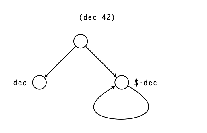
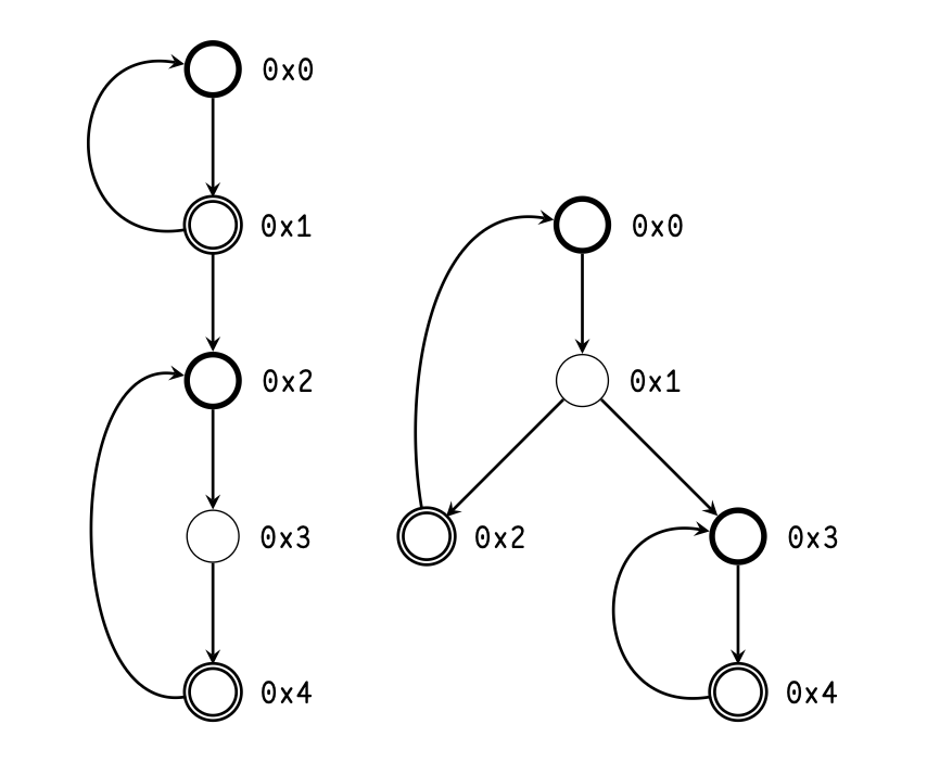
The abstract call graph may contain cycles. Figure 1 shows the abstract call graph for Nock obtained from compiling (dec 42) against ..ride subject. Firstly dec expression is evaluated, which pulls +dec arm from a core in the subject. With the product of that expression, which is the dec core, pinned to the subject, we edit that core with the argument 42, then we pull the arm $ from that core. The $ arm call either returns the decremented value or calls itself, incrementing the counter.

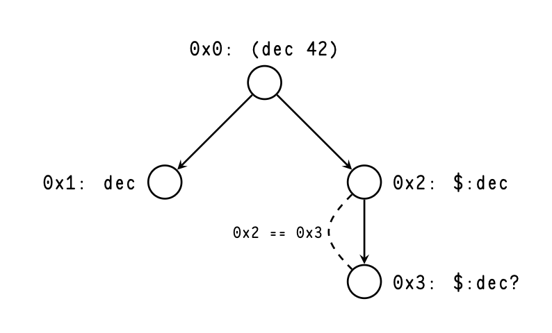
When we traverse that call graph, we cannot simply follow the edge from $:dec to itself, as doing so would cause an infinite loop in the algorithm. Instead, when we detect a loop call, or a backedge, we immediately return an unknown result from the child call. As we traverse the call graph, we enumerate the vertices, as shown in Figure 2.

Figure 2 also demonstrates that the ska representation of the call graph is acyclic: back-pointing edges are replaced with a forward-pointing edge to a new vertex that we do not analyze through. Together with the fact that both branches are traversed in Nock 6 analysis, ska call graph traversal becomes a genuine depth-first, head-first traversal.

5.3 Loops as strongly connected components

From the point of view of the abstract, cyclical call graph, a set of functions that cannot be finalized unless all functions from this set are finalized forms a strongly-connected component (scc) of that call graph. Thus, handling of loops in ska becomes a question of handling sccs. The algorithm that follows was developed by the author to detect and manage sccs during the analysis. The process turned out to be quite similar to Tarjan’s 1972 algorithm for finding sccs with some differences:

• In Tarjan’s algorithm, the graph is known ahead of time, while in ska the graph is simultaneously inferred with symbolic execution of Nock and traversed.

• Since Nock call graph is rooted, only one traversal is necessary, and in this traversal the descendants down the non-loop call edges are guaranteed to have higher index values.

The latter fact allows for simpler comparisons and simpler state management, allowing to have a stack of sccs instead of a stack of vertices that are popped when an scc is finalized. For example, when returning from a vertex which is a member of a non-trivial scc in ska we only have to check one boolean value and compare the index of this vertex with the index of the entry of the current scc with equality operator, so we do not have to call arithmetic functions and pay Nock function call overhead.

As the call graph is traversed, we keep track of the stack of mutually independent sccs (that is, sccs whose unions are not sccs) by keeping track of the entry point (the earliest vertex that has a backedge pointing to it) and the latch (the latest vertex that has a backedge originating from it).

Suppose that we encounter a new backedge. To determine whether it forms a new scc, or belongs to an already existing one, it is sufficient to compare the parent vertex enumeration label with the latch of the latest scc on the loop stack. If the parent vertex is greater than the latch, a new scc data structure is pushed on the stack; otherwise, the top scc’s entry and latch are updated, and then that scc is repeatedly merged with the one beneath it if the connection condition is satisfied: the entry of the updated scc is less than or equal to the latch of the preceding scc.

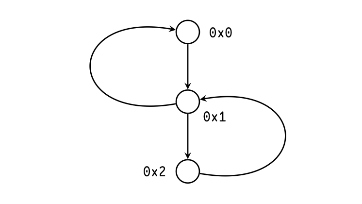
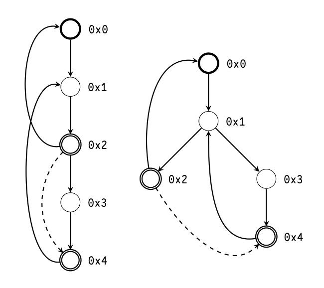
Let us prove that this comparison is sufficient. Recall that the enumeration labels are assigned in depth-first, head-first order. If the backedge parent is equal to the latch of the scc, the kid is a part of the scc since the kid is reachable by an scc member, in this case, the parent, and a member of scc is reachable from kid via the backedge (Figure 3).

If the parent label is greater than the latch, then either they are on the same root path or not. In both cases, no member of the scc can be reached from the parent, making the parent, kid, and all vertices in between a new scc. These scenarios are illustrated in Figure 4.

Finally, if the parent label is less than the latch, then either they are on the same root path or not.

If they are, the latch is the parent’s descendant, making the latest scc reachable from the parent. Since the parent and the kid are necessarily of the same root path, which makes the kid reachable from the latch, making both the parent and the kid vertices reachable from the scc, thus making the kid, parent, and all vertices between them are part of the previous scc.

If they are not, then the latch still has to be a parent’s descendant. Let us sketch the proof by disproving the contrary.

Suppose that the opposite is true. Then the parent vertex is to the left of the latch, where “A is to the left of B" means that A is entered before B and A is not B’s predecessor. The latch is either on the same root path as the kid or it is to the left of the kid vertex, since the latter is the latest vertex we discovered. Since “leftness" is transitive, that means that the parent is to the left of the kid, which is impossible since they are on the same root path. Contradiction: the latch and the parent are on the same root path, making the kid, parent vertices, and vertices between them parts of the existing scc. Illustrations for both scenarios are shown in Figure 5.

The condition for scc merging in case of scc extension is the same. In fact scc extension can be represented in terms of scc creation, together with merging with the topmost scc in the loop stack.

5.4 Cycle Validation, Code Usage Distribution, Fixed-Point Search

Since loop validation is deferred until returning from the loop entry point, subject usage by the loop calls is not recorded until that point. At loop validation, we want to distribute subject code usage information of the parent over the kid’s subject provenance, finally making an update we deferred so far. But by doing so, since the kid’s subject may contain nouns from the parent call, given that the kid is always a parent’s descendant in the call graph, we might update usage information of the parent’s subject. We would have to do that in a loop until the parent’s subject usage converged to the fixpoint value for that transformation.

For each backedge that we are validating, we perform the following steps:

1. We calculate the parent subject, masked down with the subject code usage information.

2. We distribute the $cape of that masked subject using kid provenance information.

3. We recalculate the new masked-down parent subject.

4. We compare their $capes. If they are equal, the fixpoint is found; otherwise, return to step 2.

5. Check masked-down parent subject and kid subject for nesting. If they nest, the backedge is valid; otherwise, the assumption was wrong, and we will redo the analysis of the loop with this parent-kid pair added to a blacklist.

Steps 1 and 3 are necessary because otherwise, if we distribute just the subject code usage information $cape without using it to mask actual data, the $cape could start growing infinitely deep, causing an infinite loop in the fixpoint search. Step 4 works because the $cape distribution along the given provenance is idempotent.

6 Performance: load-bearing design choices and optimizations

6.1 Vastness of nouns

It is important to have a sense of scale when dealing with ska. Consider, for example, Urbit’s standard library core zuse. How many nouns are there in total in that library? In Arvo 409K:

> =/  n=*  ..zuse 
  |-  ^-  @ 
  ?@  n  1                    ::  atom is one noun 
  ~+                          ::  %memo hint 
5  +((add $(n -.n) $(n +.n)))  ::  cell is 1 noun + 
                              ::   nouns in head + 
                              ::   nouns in tail 
1.656.521.503.863.284.811.637

This yields \(1.66 \times 10^{21}\) nouns! “Billions of billions" would be an underestimate.

But Urbit’s runtime, Vere, handles this mass of nouns just fine. We can estimate that it takes only about 1.2 MB to store that library. What is going on? And how can anything calculate the number of nouns in a reasonable time with something that looks like naive tree traversal?

The answer lies in structural sharing.³ The standard library supplies many duplicated nouns, which are represented as pointers to reference-counted data structures. The reason we could count the number of nouns with something that seems like a simple tree traversal is the use of %memo hint that enables memoization of Nock results, using the subject-formula pair as a key. Even if the nouns are large, their comparison is still fast precisely because they are duplicated: noun equality check is short-circuited on pointer equality. So even though pointer equality is not exposed in Nock directly, having nouns be pointer-equivalent is crucial for performance. Thus, when developing algorithms with performance in mind, we need to:

1. Make sure not to disrupt structural sharing whenever possible;

2. Leverage structural sharing by either short-circuiting various checks/comparisons with Nock 5 equality test, or by using Nock memoization.

6.2 Provenance Tree

We represent the provenance information of the subject with $source:

+$  source  (lest (lest *))

where lest is a non-empty list.

Raw nouns in the inner list describe the provenance from a function call’s subject to a use site of that noun. The value can be one of:

• 0, if the noun does not come from the subject, e.g., it was created. by evaluating Nock 1 from the formula;

• a non-zero atom, in which case the noun comes from the given axis of the subject.

• a cell, in which case the noun in question is also a cell, and its head and tail have provenances that are described by the head and tail of the provenance noun respectively.

Nock 1, 3, 4, 5, and 12 erase provenance information. Nock 0 gets a sub-provenance tree in an obvious way. Nock 7 composes the provenance calculation. Nock 10 performs an edit. All are similar to the $sock treatment. What differs significantly is the handling of the branching operator Nock 6. What we care about is where the data could come from, so we need to calculate a union of provenances, masked down to the intersection of produced data. Instead of creating a tree that includes all union information, in the spirit of saving structural sharing, we simply make a list of simple provenances. Thus (lest *) is a union of provenances in a given call.

The outer list keeps entries per call frame. Whenever we enter a new call with Nock 2, we push the new provenance union list ~[1] onto the provenance stack. When we return from a call, the stack is popped, and the popped provenance union list is composed with the second-to-top. Whenever we need to distribute subject usage, e.g., when we encounter a direct call, the provenance stack is folded with composition.

6.3 Provenance tree operations and heuristics

When dealing with provenance information $source, some heuristics were added to improve performance. When applying binary functions like composition to two union lists of provenances, the function would be applied to all pairs, and a new union list would be constructed, omitting duplicates or other provenances that nest under some other provenance that is already present in the assembled list. The compatibility check function only checks provenance nouns up to ten cells deep, assuming that they are incompatible beyond that point. This heuristic prevents from walking provenance nouns exhaustively and taking too much time if they are too deep at the expense of possibly having larger union lists with duplicates, which does not affect the semantics of the algorithm. In case of Nock 10 provenance edit, the check was disabled altogether if the lengths of the union lists of donor and recipient nouns multiplied exceeded 100.

Since the provenance union is expressed as a list, there are two ways of implementing the consing of provenances. We can either cons every member of the list of the head provenance with every member of the list of the tail provenance, yielding a union list with the length equal to the product of the lengths of the operand lists. Alternatively, we can cons every member of the list of the head provenance with empty provenance 0, cons 0 with every member of the list of the tail provenance, then concatenate the lists. That way, we end up with a union list whose length is a sum of the operand lists’ lengths. The algorithm for consing chooses between two approaches depending on the length of the operand lists, using the multiplicative approach almost always, since typically the union list length is one, and switching to the additive “cons via union" if the union lists are too long.

6.4 Load-bearing comparison checks and %memo hints

In $cape and $sock arithmetic, equality check shortcuts for $cape union, which is heavily used for code usage information updates, and $sock intersection, which is used for Nock 6 product calculation, are load-bearing. For %memo hints, we use them to short-circuit Nock memoization hints, these are load-bearing for provenance noun composition and construction of subject capture mask used for in-algorithm caches described below. They also appear to add marginal performance improvements in other places of the algorithm in case of backtracking (reanalyzing a cycle over and over due to making incorrect guesses).

6.5 Algorithm caches for finalized and non-finalized calls

To prevent doing the same work over and over, we want to cache the intermediary analysis results. For finalized calls, the cached data includes the formula and the minimized subject, where the latter includes potential subject capture in addition to code usage. If a Nock 2 formula gets a cache hit, it updates the code usage information using the mask from the cache, and returns the product, which it constructs by taking the cached product $sock and composing the cached union list with current subject provenance, effectively applying the provenance transformation of the cached call to the new subject.

Caching finalized calls turned out to be not enough, as demonstrated by ~ritpub-sipsyl and ~master-morzod.⁴ To prevent reanalysis of cycles in highly mutually-recursive code like the Hoon compiler, caching of non-finalized calls was also necessary. Similarly to finalized-call caching, a potential cache match would check the subject it has for nesting with the cached subject $sock, masked down at cache check time with the currently available code usage information. Similarly to loop calls, the code usage information distribution along the new subject provenance would be deferred to the cycle validation. Another point of similarity is the necessity of checking cycles for overlap and merging in case they do, since a cache hit call would have a loop call to a member of an scc to which the cached function belongs.

Unlike loop calls, the fixpoint search is not necessary since the cached call and the cache hit are never on the same root path, so distributing the code usage information along the hit call subject provenance would never have an effect on cached call. Validation is still necessary, and reanalysis of cycles due to incorrect non-finalized call cache guesses is currently the biggest overhead in the analysis.

7 Vere integration

The integration of ska analysis into Vere was done in the simplest imaginable way as a proof of concept. The road struct was updated to include bytecode caches for ska-produced code and to house the analysis core. A new static hint %ska marks the entry point into the analysis-compilation lifecycle.

7.1 Nomm (Nock--)

In addition to producing call graph information, the ska algorithm also produced desugared, annotated Nock-like code called Nomm (a sort of Nock--). The practical difference, apart from Nock 9 and Nock 8 expanded into other Nock operators, is the annotation data in Nock 2. The version of Nomm that is provided for use with the Vere development fork with ska, $nomm-1, is mostly indistinguishable from $nock proper:

+$  nomm-1 
  $^  [nomm-1 nomm-1] 
  $%  [%1 p=*] 
      [%2 p=nomm-1 q=nomm-1 info=(unit [less=sock fol=*])] 
      [%3 p=nomm-1] 
      [%4 p=nomm-1] 
      [%5 p=nomm-1 q=nomm-1] 
      [%6 p=nomm-1 q=nomm-1 r=nomm-1] 
      [%7 p=nomm-1 q=nomm-1] 
      [%10 p=[p=@ q=nomm-1] q=nomm-1] 
      [%11 p=$@(@ [p=@ q=nomm-1]) q=nomm-1] 
      [%12 p=nomm-1 q=nomm-1] 
      [%0 p=@] 
  ==

In the case of %2, info=~ denotes an indirect call, and a non-empty case denotes a direct call with a known formula and masked subject. The pair of a minimized subject and a formula is used here as a unique identifier for a Nomm function.

7.2 Road data structures

Two hamt tables were added to the u3a_road struct: dar_p, a map from [sock formula] pair to loom offset of u3n_prog bytecode u3p(u3n_prog), and lar_p, a map from formula to a list of pairs [sock u3p(u3n_prog)]. The former is used during Nomm compilation to bytecode, the latter is used for searching for bytecode with direct calls, given a formula and a subject.

The Nock bytecode struct was extended with an array of direct call information structs:

/* u3n_dire: direct call information 
 */ 
typedef struct { 
  u3p(u3n_prog)  pog_p; 
5  u3j_harm*      ham_u; 
  c3_l           axe_l; 
} u3n_dire;

where

• pog_p is a bytecode program loom offset for the direct call,

• ham_u is a nullable pointer to a jet driver if the jet match occurred at compile time,

• axe_l is the arm axis for jet driver debugging checks.

Another addition to the road struct was a field for the analysis core +ka. A jammed cell of four pre-parsed Hoon asts for ska source files was added to Vere source code, which was unpacked and built into a core when the ska entry point was executed with +ka core not being initialized.

7.3 Analysis lifecycle

Let us follow the execution of a [subject formula] pair using ska. It starts with annotating a computation with a %ska hint:

~>  %ska

7.3.1 %ska hint

When the regular bytecode compiler in Vere encounters a %ska hint, it defers the compilation of the hinted formula and emits ska-entry point opcode. When that opcode is executed, a lookup is performed in lar_p, returning u3n_prog* on success. If the lookup failed, the pair of subject and formula is passed to +rout gate of the +ka core, which returned +ka core with global code tables and cold state updated. After that, the code maps were extracted from the global state, and the ska compiler function was called with the subject, formula, and the maps as arguments. The maps include:

• cole: a map from [sock *] to [path axis] for cold state accumulation,

• code: a map from [sock *] to loom offset of u3n_prog for finalized call caching,

• fols: a map from formula to a list of pairs [sock u3p(u3n_prog)] for non-finalized call caching.

7.3.2 Nomm compilation and execution

The main difference between compiling regular Nock to Vere bytecode and compiling Nomm is that compiling a Nomm formula with direct calls also requires compiling all its callees recursively. A rewrite step was added to handle cycles properly: on the first pass u3_noun values for [sock *] pairs were saved in u3n_dire structs, and on the second pass, these values were replaced with corresponding u3p(u3n_prog) values.

Once the bytecode program for the entry point function and all its descendants were compiled, the Nock bytecode interpreter would execute this program as any other program, with the only difference of having direct call opcodes that skip bytecode cache lookup and jet matching.

7.4 Benchmarks and Notable Results

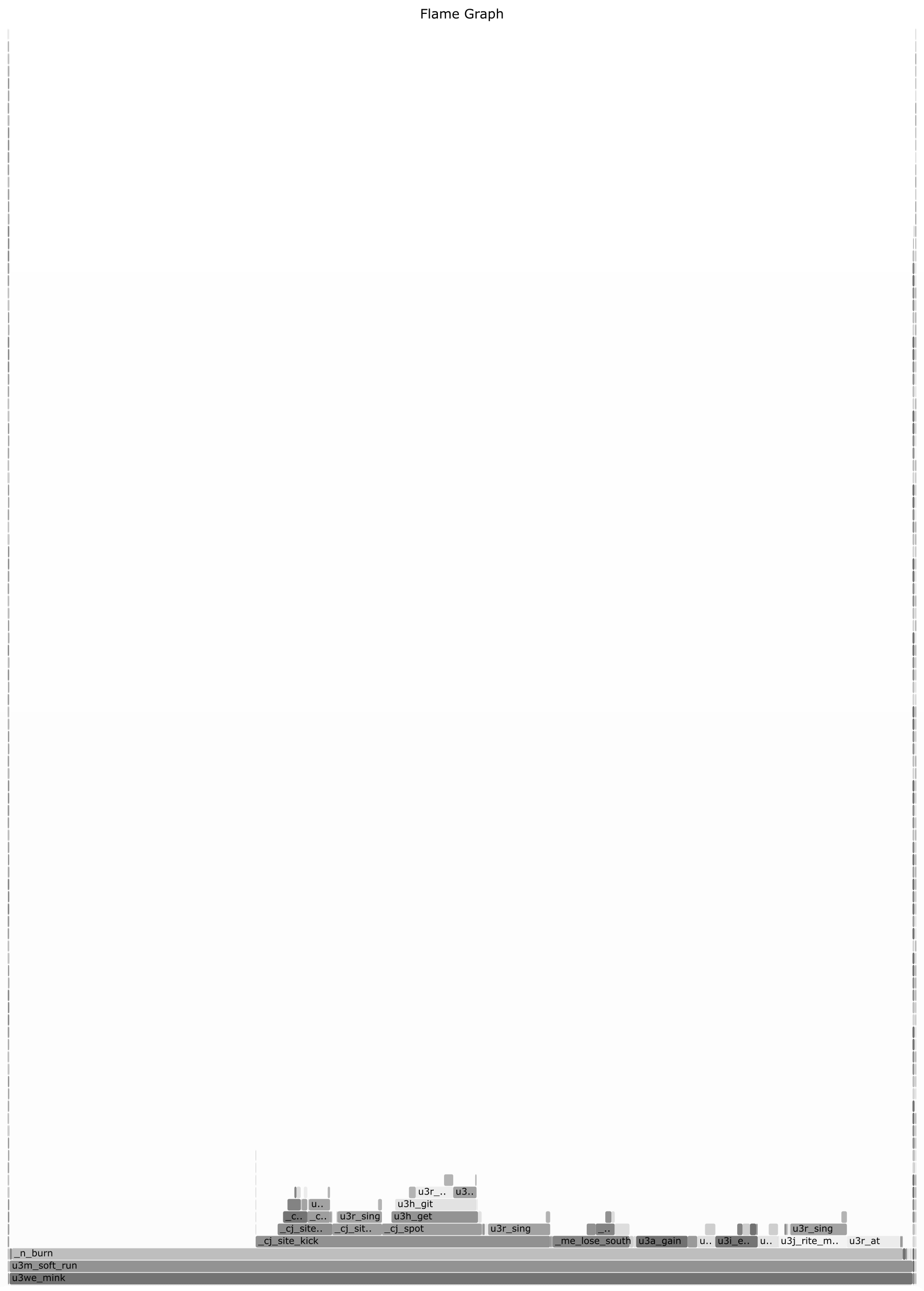
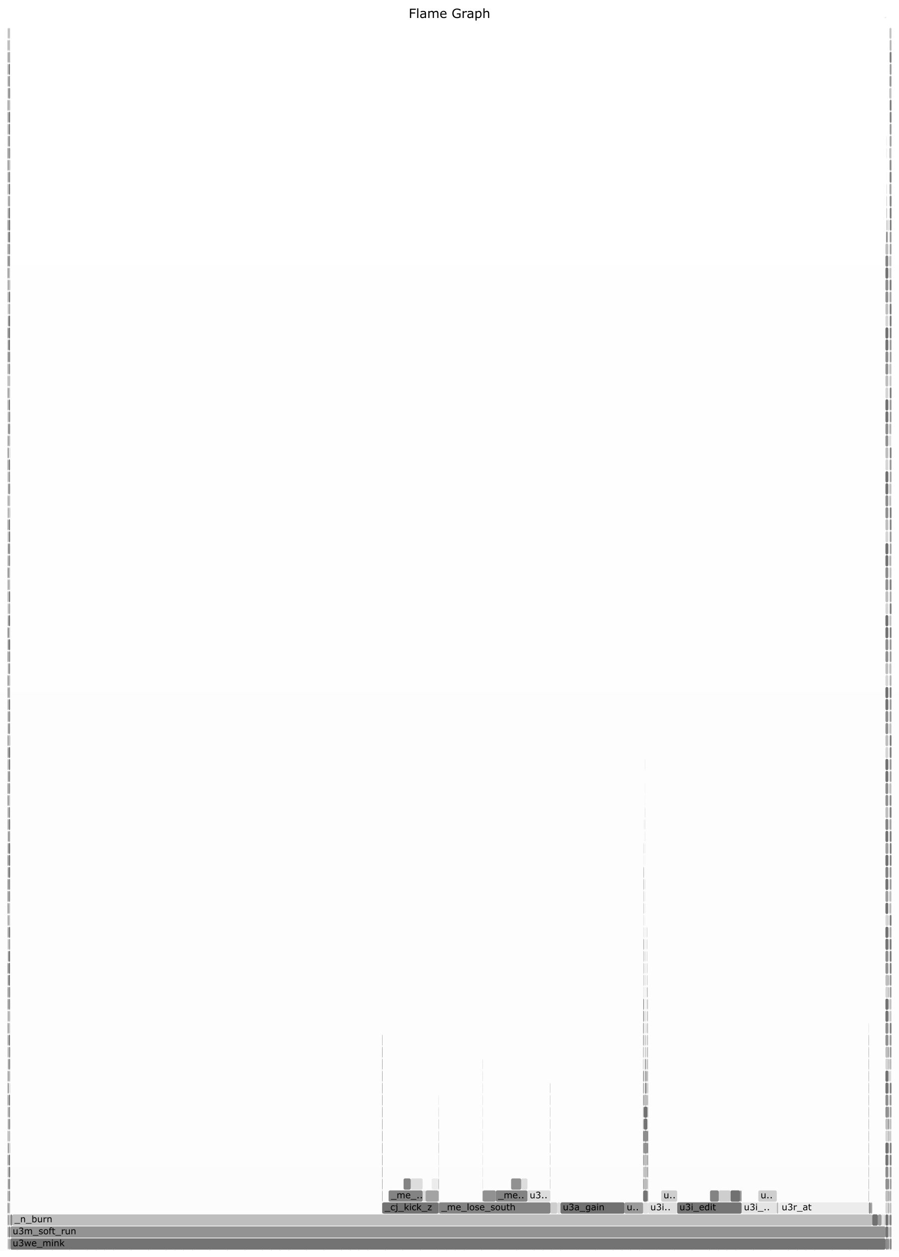
The effect of the %ska hint on performance was compared for the Ackermann function and a simple list iteration algorithm. In both cases, the performance gain was around 1.7\(\times \). The main overhead in computations with direct calls appears to come from refcounting/ allocating/freeing operations and interpretation (Figures 6 and 7).

When it comes to the performance of the ska algorithm itself, the results were sometimes surprising. Paradoxically, analyzing +mint:ut call itself took ~m1, while analyzing the entirety of hoon.hoon, including +mint:ut, takes ~s13. The reason appears to be a lack of knowledge in the solo +mint:ut call case, causing excessive backtracking due to wrong non-finalized call cache hits (thus validating ska’s fundamental thesis). In addition, every time the loop analysis was discarded, all caches were also discarded, leading to making more work multiple times when compared to the hoon.hoon case. In the latter case, no wrong cache hits were made.

8 Conclusion and future work

There appear to be two viable future directions for this project. A short-term objective is a proper integration with the Vere runtime, such as making compiled ska bytecode caches persistent and integrating cold states of Vere and ska. A longer-term direction would pursue ~ritpub-sipsyl’s original vision by implementing ssa ir compilation, which would ameliorate allocation overhead caused by cell churning⁵ during temporary core construction for calls and deconstruction to get function arguments.

References

Tarjan, Robert Endre (1972). “Depth-First Search and Linear Graph Algorithms.” In: siam Journal on Computing 1.2, pp. 146–160. doi: 10.1137/0201010. url: https://epubs.siam.org/doi/10.1137/0201010.

Footnotes